

Introduction
Image generation is a compute-bound problem which requires accelerated hardware to be viable for commercial use cases. Most inference providers look to NVIDIA GPUs, particularly the Blackwell, Hopper, Ampere, and RTX architectures, to serve such models. The high cost of these chips, though, presents a unique opportunity to generate better margins by looking to alternative hardware which offers more FLOPs per dollar, in particular AMD’s Instinct architecture. We show that using the Luminal compiler, competitive inference latency can be retained while reducing inference costs significantly (> 40%.)
The issue that presents itself revolves around AMD’s software stack. While ROCm has made many improvements since its initial release in 2016, it is still generally regarded as inferior to CUDA. The general consensus is that AMD achieves lower realized TFLOPs at inference time, erasing the margins to be made from the lower cost of AMD chips. This keeps many providers from making the transition to AMD, despite the opportunity for vastly better margins. Furthermore, such a transition usually requires hiring kernel engineers with expertise in a specific chip manufacturer’s software stack, in this case AMD… a nontrivial barrier to diversifying across hardware architectures.
As we will show, using the Luminal ML graph compiler we can achieve highly competitive performance for image generation on AMD MI300X chips, which translates to significant cost savings for inference providers. The MI300X finishes an image 31% to 16% behind an H200 depending on resolution, while renting for less than half the price. Per image, that works out to 41% to 47% cheaper.
Background
E-graphs
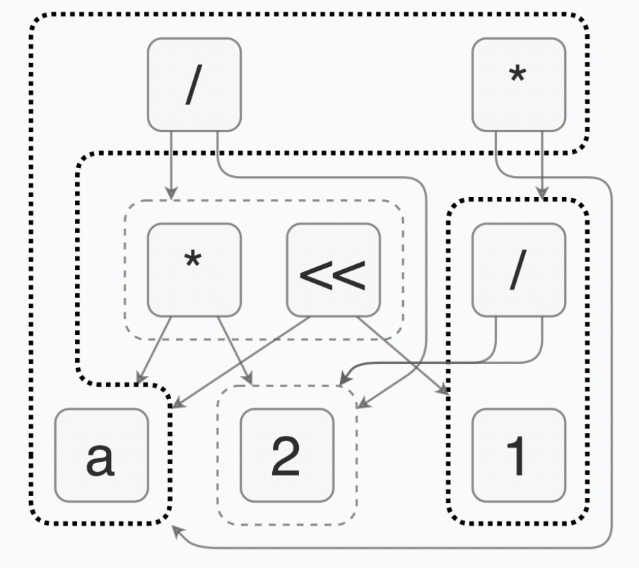
An e-graph is a data structure for compactly representing a set of equivalent expressions (programs). More concretely, if we think of an ML program as an expression which defines its output(s) in terms of its input(s), then an e-graph compactly represents a set of equivalent expressions.
Two components form an e-graph: e-nodes and e-classes. E-classes are composed of e-nodes which represent interchangeable terms of an expression, and each e-node points (via an edge) to a subsequent e-class.
The usefulness of such a representation is that one will always form a valid expression (program) by doing the following:
Begin at the root e-class of an expression.
Select any e-node from the e-class.
Follow the directed edges from that e-node to the e-classes it points at.
Repeat steps 2 and 3 until arriving at leaf nodes.
The common example that many find useful is to think about the expression (a*2)/2. More specifically the reader should think about its representation as a postfix expression: a 2 * 2 /.
Equality saturation and egglog
Given some original expression (program) and a set of rules, equality saturation is the process by which an e-graph is populated to form many equivalent expressions.
Going back to the earlier (a*2)/2 example, a useful set of rules would be:
x*2 → x«1(x*y)/y → x (y≠0)x/x → 1 (x≠0)x*1 → x
An important quality of equality saturation is that original expressions are kept as rewritten expressions are added to the e-graph. For example if we applied a sequential (destructive) rewrite a*2 → a«1, we would miss the opportunity to cancel out 2/2 to arrive at the simplified expression a.
egglog is the domain-specific programming language that we use to express rewrite rules and perform equality saturation over arbitrary expressions.
The Luminal compiler
The core insight at Luminal is that ML graph compilation, the process by which ML models are lowered from a high-level representation like that in PyTorch down to an executable program that runs on heterogeneous hardware, can be treated as a search problem. Our compiler leverages egglog and e-graphs to take a generic representation of an ML model and lower it down to optimized kernels for a specific hardware backend.
The optimizations the Luminal compiler forms are two-fold. The simple rewrites apply basic algebraic properties, constant folding, and layout canonicalization. The more interesting rewrites, however, are the hardware backend-specific rewrites. In the context of AMD, some example rewrites might be conceptualized as follows: “this scatter-multiply-sum operation is a matrix multiply which matches a hipBLASLt kernel”, “this matrix-multiply, scale, softmax, matrix multiple combination is an attention op that can be lowered to this fused flash attention kernel”, or “these primitive operations represent a convolution which can be lowered to this tiled convolution kernel.” Notably, every rule adds an alternative to the e-graph without replacing the pattern a particular rewrite matched on. This enables our genetic search algorithm to progress towards globally optimal expressions (programs.)
Luminal’s compiler approach to inference has two primary advantages. First, optimizing models to run in a commercially-viable manner becomes an automated process with our compiler. With the Luminal compiler, model optimization no longer requires dedicated kernel and inference engineers. Second, the friction of moving inference from one hardware stack to another is greatly reduced with our hardware-agnostic compiler.
Flux.2 Klein 9B

The Flux.2 family of models provides unified image generation and editing for various commercial applications. In our case, we use Flux.2 Klein 9B and compare model performance on an NVIDIA H200 and an AMD MI300X.
Flux.2 Klein 9B supports text-to-image and image-to-image pipelines; we perform our benchmark using the latter. The image-to-image pipeline consists of four components: a VAE (variational autoencoder) image encoder, a Qwen3 8B text encoder, the multi-modal diffusion transformer itself, and a VAE image decoder. All weights are stored as bf16.
The input image is encoded by the VAE into a latent space which downsamples the height and width 16 times and expands the RGB channels to 128 different channels in the latent space. The image tokens represent non-overlapping patches in this latent space.
The text encoder takes the hidden states from the ninth, eighteenth, and twenty-seventh layers of the text encoder and concatenates them to form a 12,228 element vector per token.
The transformer consists of eight double-stream blocks and twenty-four single-stream blocks. (The core difference between a double-stream and single-stream block are the projections before the attention mechanism and the normalization layer and feed-forward network after it. I highly recommend reading this paper to better understand the Flux architecture.) The hidden dimension’s size is 4,096 and the transformer has thirty-two attention heads.
Klein 9B uses guidance-free, step-distilled diffusion to deliver low latency image editing. The diffusion stage of the pipeline runs in four steps, and because the model is distilled there is no classifier-free guidance and therefore no second forward pass per step.
Setup
Flux.2 Klein 9B’s performance on an H200 and an MI300X was compared using three differently sized input images and accompanying prompts. For each pair of input image and text prompt, we ran five warmup runs and then measured 100 end-to-end runs. Each scenario outputs an image the same size as its input.
We used the following configurations for comparison:
512x512; “add a boat to the water”.
704x864; “add a hot dog stand in the background”.
1200x800; “give the dog wings”.
Both setups use the same seed (42), four diffusion steps, a 512-token padded prompt, batch size one, and bf16 weights throughout. Timing on both sides is measured with a device synchronize at every stage boundary, so the per-stage numbers are wall-clock and nothing is hidden by asynchronous execution. Model loading, compilation, and warmup are excluded from the timed runs on both sides, as is writing the output PNG. A serving process pays those costs once at startup, so folding them into per-image latency would describe a cost production never pays.
The NVIDIA H200 pipeline
The Nvidia H200 pipeline uses torch.compile with max-autotune enabled for the reference encoder, text encoder, and decoder sections. The diffusion transformer is compiled using Nvidia’s TensorRT backend to deliver maximum runtime performance, only short of handwriting kernels specific to the Flux.2 Klein 9B diffusion transformer.
To construct the entire pipeline, we use the Diffusers Flux2KleinPipeline and its Flux2Transformer2DModel, AutoencoderKLFlux2, and Hugging Face Qwen3ForCausalLM components, running on PyTorch 2.7 with CUDA 12.6.
The H200 pipeline makes the following optimizations:
A static TensorRT engine for the transformer. The Diffusers
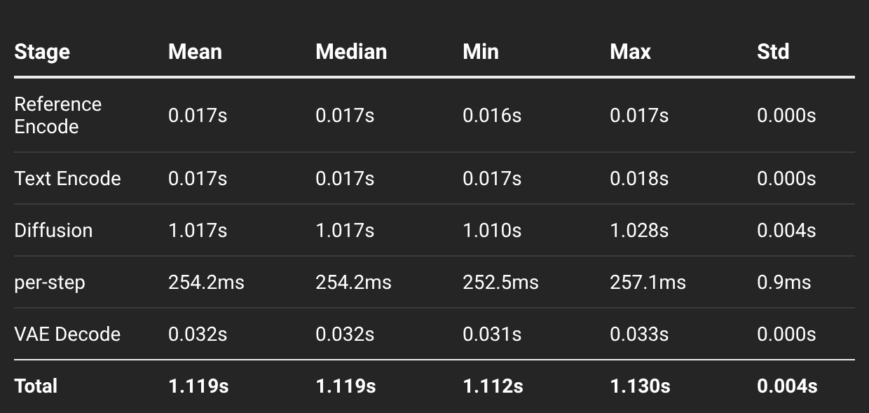
Flux2Transformer2DModelis exported to ONNX with PyTorch’s dynamo exporter and built into aTensorRTengine. This is the NVIDIA-side analogue of Luminal’s compile-and-search step: a shape-specialised program, with the search done by TensorRT’s tactic selection.What the engine runs per step. TensorRT’s own runtime enqueues the engine directly on the PyTorch stream. Each diffusion step is 433 kernel launches: 115 Hopper XMMA GEMMs, 32 fused multi-head attention kernels, and
TensorRT’s fused elementwise code. Across the run the GEMMs take 58% of GPU time, the attention kernels 23%, and the fused kernels 13%, with a step averaging 252 ms and the GPU busy for about 97% of the run.Fixed-shape everything. Prompts are always padded to 512 tokens, width and height must be multiples of 16, and the engine is built for exactly one token count; a different output size derives a different engine file and a rebuild. Static shapes are what make max-autotune, CUDA graphs, and a single-profile engine viable.
Fused attention at every site. Inside the engine, all 32 transformer attention sites run through TensorRT’s fused attention kernel at about 1.9 ms per call, roughly a quarter of each step. In the text encoder, PyTorch’s scaled_dot_product_attention dispatches to the CUTLASS memory-efficient attention kernel inside the Inductor graph, once per Qwen3 layer. The VAE mid-block attention takes the same path in the encoder and the decoder.
The AMD MI300X pipeline
The MI300X examples run using Luminal’s ROCm backend. The different components of the Flux.2 Klein 9B pipeline are written in Luminal’s high-level graph language (the transformer, the Qwen3 text encoder, and the VAE encoder and decoder are all Luminal graphs), and the compiler lowers each of the four stages to a program specific to the MI300X. The Luminal high-level graph is a generic model spelling: there are no references to kernels, libraries, or layouts. The compiler choses all of these itself. The compiler’s ROCm lowers to the following:
hipBLASLt for matrix multiplies, AMD’s equivalent of cuBLASLt, with bias epilogues fused into the GEMM where the compiler can prove the layout allows it. All
bf16GEMMs accumulate infp32.Fused attention. The compiler identifies fused flash-attention kernels that compute
softmax(QK^T)Vin a tiled fashion, maximizing realized FLOPs. Both the text encoder and diffusion transformer make use of such a kernel.Tiled convolution kernels. Similar to the fused attention, tiled convolution kernels are dispatched to, by shape, at runtime. Said kernels are always ahead-of-time compiled based on the shapes the compiler identifies in the ML graph.
Fused RoPE, RMSNorm, and LayerNormModule kernels. As opposed to launching separate GEMM kernels and reduction kernels, each of these operations is launched as one fused kernel to save on kernel launch overhead.
Generated HIP kernels for everything else: fused elementwise chains, reductions, gathers, casts. The compiler identifies regions of the ML graph which can be fused together into a singular kernel.
HIP graphs to batch kernel launches. Each transformer step is 33 HIP graph launches interleaved with 32 attention calls, rather than roughly 1,250 individual kernel launches.
Runtime execution is otherwise uneventful: the four stages run back to back, the Euler sampler integrates the latent on the host in fp32, and the reference latent is computed once per run and appended to the noise tokens.
It should be noted that the entire compilation of the pipeline (effectively four separate compilations), the phase where Luminal performs it’s kernel search, takes a few minutes. While not insignificant, this cost is payed up front across the five warmup and one-hundred timed runs. In a production setting, the cost of compilation would be negligible as it is amortized across inference requests.
Results
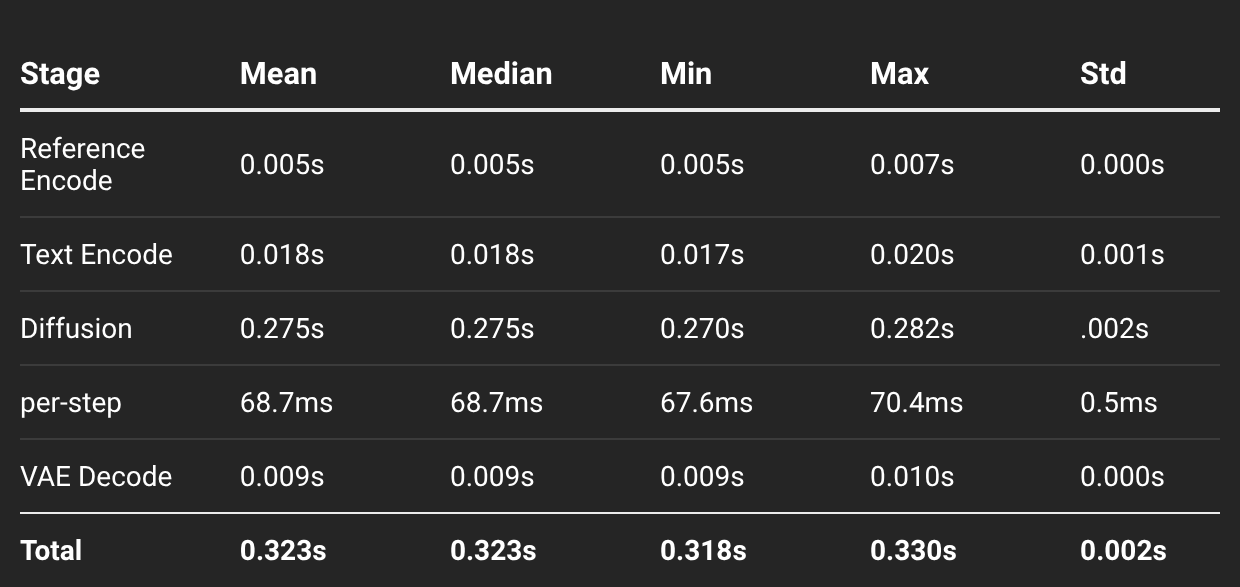
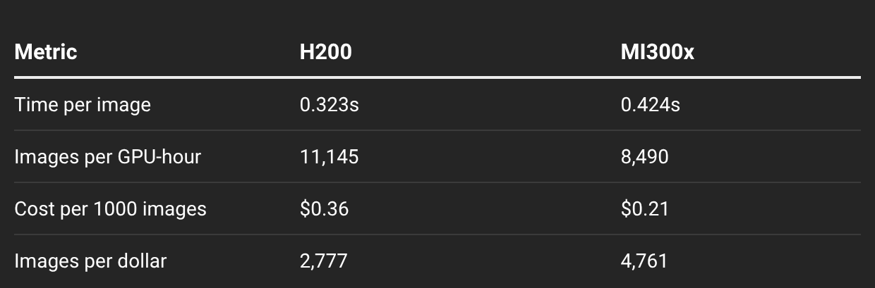
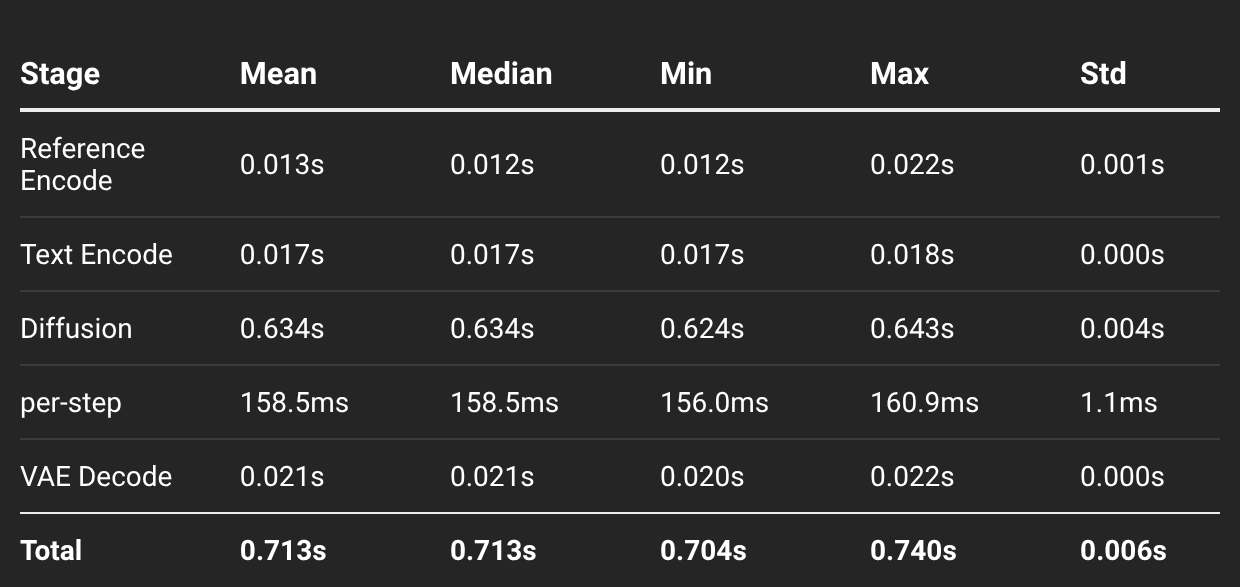
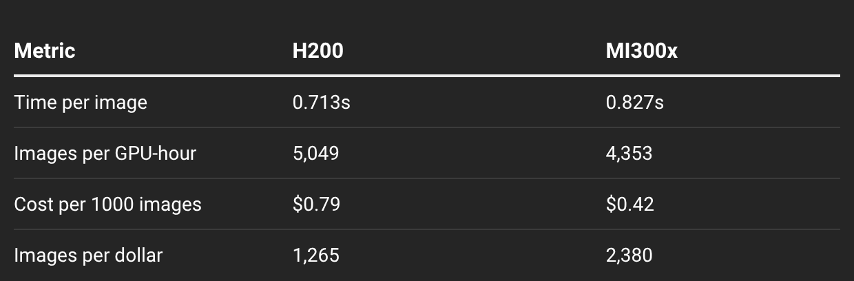
Each configuration shows the input image, the H200 output, and the MI300X output side by side, followed by the per-stage timings on each GPU and the cost comparison. Costs use $4.00 per GPU-hour for the H200 and $1.85 per GPU-hour for the MI300X.
Configuration 1: 512x512, “add a boat to the water”



NVIDIA H200 (PyTorch, TensorRT):
AMD MI300X (Luminal):
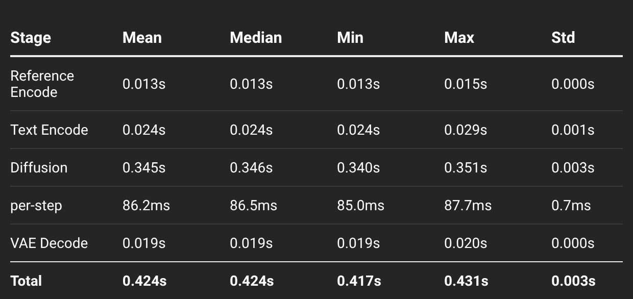
The MI300X takes 31% longer per image and costs approximately 41% less per image.
Configuration 2: 704x864, “add a hot dog stand in the background”



NVIDIA H200 (PyTorch, TensorRT):
AMD MI300X (Luminal):
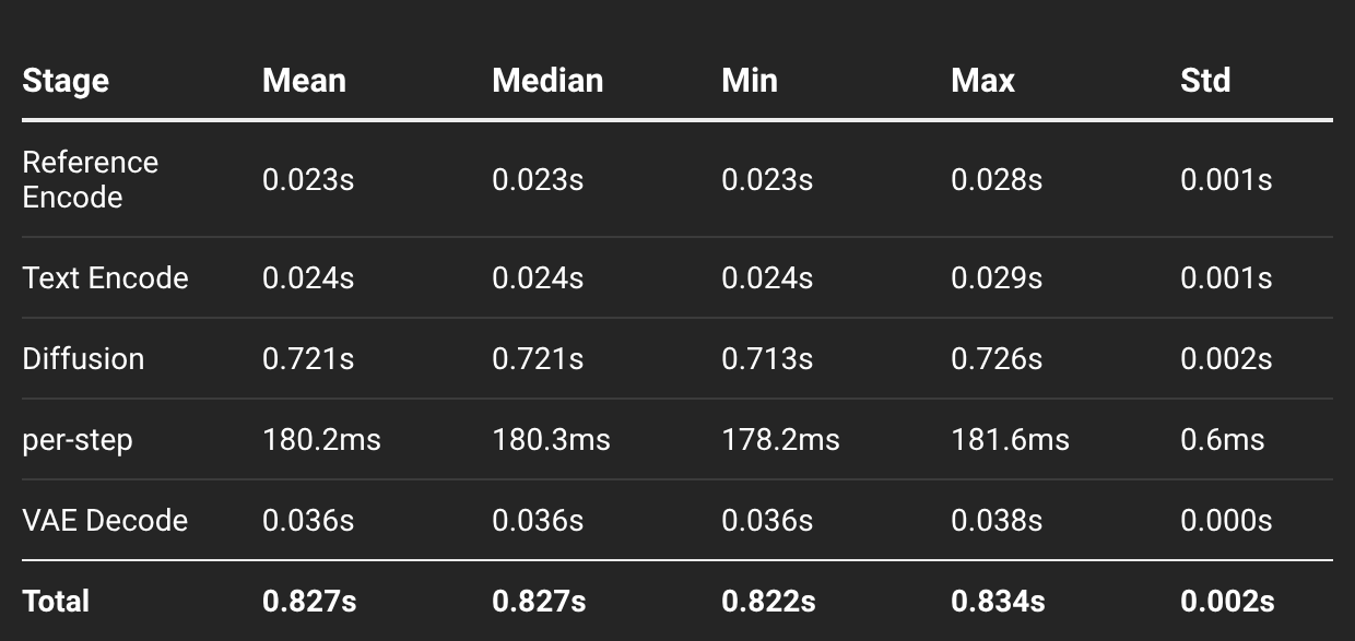
The MI300X takes 16% longer per image and costs 47% less per image.
Configuration 3: 1200x800, “give the dog wings”



NVIDIA H200 (PyTorch, TensorRT):
AMD MI300X (Luminal):
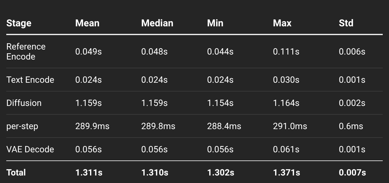
The MI300X takes 17% longer per image and costs 46% less per image.
Comparing Luminal to SGLang Diffusion
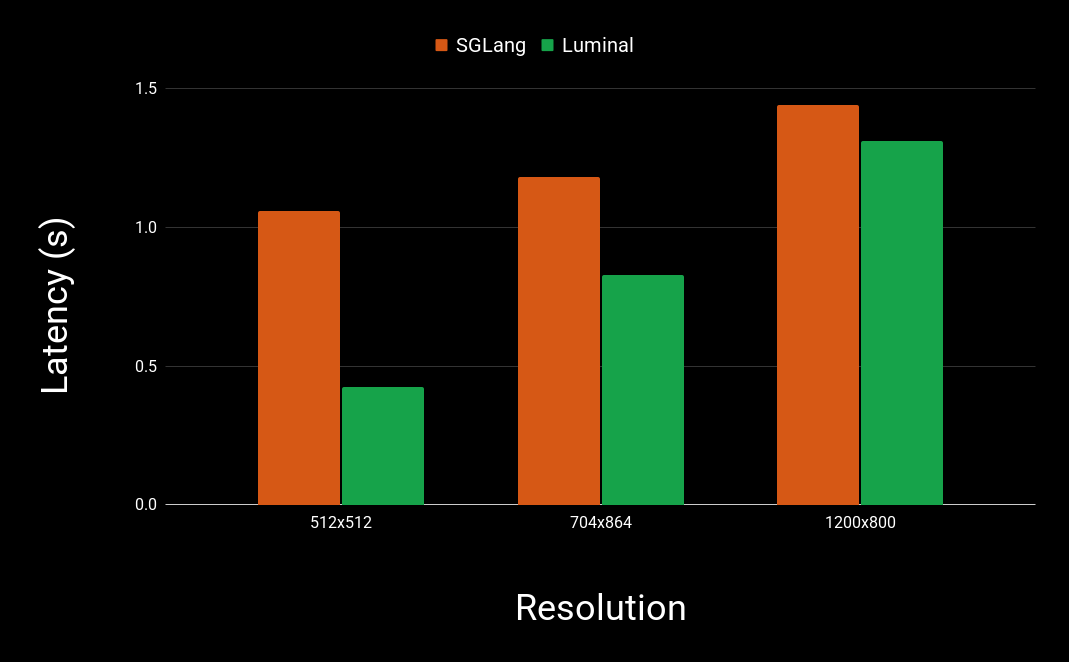
While the primary concern of our benchmark was to compare the performance the Luminal compiler delivered on an AMD MI300x as compared to an Nvidia H200 using TensorRT, we also felt it useful to compare the Luminal compiler against SGLang on the AMD MI300x.
We made the same assessment with SGLang’s multi-modal engine and benchmarked the same three images and corresponding resolutions. We only assessed offline throughput, so no latency introduced by the SGLang inference server was measured. Additionally, SGLang was configured to use torch.compile, which the inference engine does not do by default. SGLang does use ROCm’s AITER backend which dispatches out to flash attention kernels during the diffusion stage, but SGLang does not make use of fused LayerNorm+adaLN or RMSNorm+Rope kernels, unlike the Luminal compiler. The result is that the Luminal compiler outperforms SGLang on all three of the image configurations.
Luminal achieves latencies of 0.424s, 0.827s, and 1.311s on the 512x512, 704x864, and 1200x800 images respectively. By comparison, SGLang is slower at 1.06s, 1.18s, and 1.44s respectively. (It is interesting to note how the gap narrows as the image becomes larger. As the diffusion stage’s share of the latency increases, SGLang’s relative performance improves as it does optimize the diffusion stage reasonably well.)
Where the time goes on the MI300X
To understand what the compiler actually produced, we profiled the 1200x800 run with a rocprofv3 GPU kernel trace, bracketed with ROCTx ranges so that only one steady-state run is recorded and the compile and warm-up are left out.
One diffusion step on the GPU is 616 kernel executions. Of those, 249 are hipBLASLt GEMM kernels captured inside HIP graphs, 32 are fused attention calls, one per attention site, and the remaining 335 are kernels Luminal generated: 152 fused elementwise kernels, 137 fused normalization kernels, and 46 small index, cast, and constant kernels. Where the GPU time goes within a step:
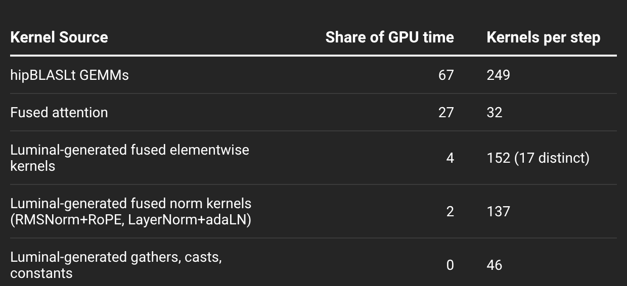
This is the profile you want for a transformer: two thirds of the time is in vendor-tuned matrix multiplies, a quarter is in fused attention, and the long tail of "glue" ops (norms, activations, modulation, RoPE, residual adds) is compressed into under three hundred fused kernels that together take about six percent. The GPU is busy for 97% of each step's wall-clock. The remaining three percent is launch gaps, most of them the ~35 microseconds pause between a HIP graph finishing and the next attention call starting.
What the compiler found on its own
The transformer, text encoder, and VAE were written as plain tensor math. Luminal’s front end has no “matmul”, “attention”, “convolution”, or “layer norm” op. It has a small set of primitives: elementwise arithmetic (add, multiply, exponent, reciprocal, and so on), reductions (sum, max), and index manipulation (gather, scatter, iota). A matrix multiply is spelled as a broadcast multiply followed by a sum. Attention is spelled as two of those, a scale, a max, an exponent, another sum, and a divide. A convolution is spelled as a gather that unfolds the input into patches, followed by a multiply and a sum. Every optimization below was discovered by the compiler from those spellings during equality saturation and search; none of it is written into the model.
Optimized GEMM kernels recognized from multiply-and-sum. The compiler matches every multiply-then-sum whose strides describe a matrix product and adds a vendor-tuned GEMM kernel to its e-class as an alternative. In the final transformer program every one of the 249 GEMMs per step went to hipBLASLt; the only generic matmuls left in the whole run are 49 tiny projections in the text encoder that together take 0.3 ms.
Flash attention recognized from seven primitive ops. The scaled-dot-product pattern (scores, scale, softmax, weighted sum) was matched at every one of the 32 attention sites, in both the double-stream and single-stream block shapes, and each one was replaced with a single fused flash-attention kernel. In the text encoder the same rules also matched the causal-plus-padding mask, which the model spells as an additive bias before the softmax. The VAE’s single mid-block attention was matched the same way in both the encoder and the decoder.
Row normalizations recognized from a reciprocal square root. RMSNorm is spelled as a square, a sum, a reciprocal square root, and a multiply; LayerNorm adds a mean and a subtract; the adaLN modulation that follows it is a scale and a shift; and RoPE is a gather of each element’s partner and a multiply-add against cosine and sine tables. Per step that is 80 RMSNorm+RoPE launches and 57 LayerNorm+modulate launches, each about 45 microseconds, and the reductions they replaced are gone from the profile entirely.
Convolutions recognized from gather-multiply-sum. The VAE spells each convolution as an unfold followed by a matrix product. The compiler proves the unfold indexing is a convolution and replaces the chain with an optimized convolution kernel: 25 of them in the encoder and 33 in the decoder, accounting for 58% and 61% of those stages’ GPU time. The zero-padding around each convolution, which the front end spells as a chain of scatters and gathers, is rewritten into a single fused select kernel that produces the padded buffer the convolution reads directly.
Elementwise chains fused into single kernels. Two fusion rules, one that grows a fused region by pulling a neighboring elementwise op into it and one that merges two adjacent regions, fired hundreds of times in the transformer stage. The result is 17 distinct fused kernels per diffusion step, launched 152 times, covering the SwiGLU activation, the gate-and-residual add after each block, the concatenation of the text and image streams, and the timestep embedding.
The claim is not that any of these optimizations are exotic or novel. A kernel engineer would think to implement every single on of these optimizations. The key point is that the compiler recognizes and chooses these optimizations from a generic spelling of Flux.2, no kernel engineer has to go in and optimize the stack. No tuning a config, no installing special attention backends, and no installing different ROCm libraries to select fused kernels from. All of this ships with the Luminal ROCm runtime.
Cost summary
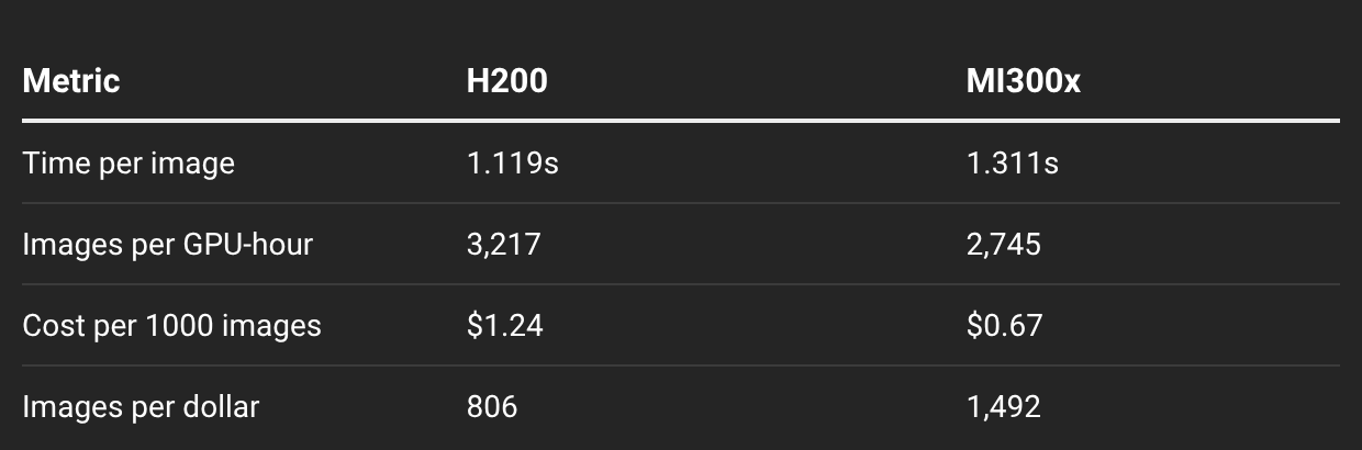
Putting the three configurations together, using $4.00 per GPU-hour for the H200 and $1.85 per GPU-hour for the MI300X:
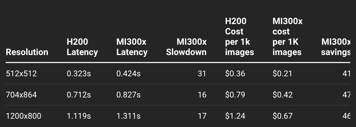
The math is simple. The MI300X rents for 46% of the H200’s price, so the break-even point is an MI300X that takes 2.16x as long per image. In practice it takes 1.16x to 1.31x as long, which leaves 41% to 47% of the per-image cost on the table. At one million 1200x800 edits, that is roughly $1,240 on H200s versus $670 on MI300Xs.
It cannot go without saying: latency matters for interactive products, and the MI300X is slower per image. That being said, for image generation workloads, latency is generally less of a concern. An additional fifth of a second is usually negligible for most products, especially considering the additional latency communication over a network introduces.
Discussion
The primary purpose of this endeavor was to assess the viability of AMD chips and the and a properly optimized ROCm stack for image generation workloads in production settings. The issue remains, however, that optimizing a ROCm stack is non-trivial for many inference providers and transitioning to AMD hardware generates a lot of friction for already time-constrained engineers.
We have shown, however, is that the Luminal compiler can absorb a lot of this friction and compile an image generation pipeline, in our case the Flux.2 Klein 9B pipeline, that is competitive from a latency perspective with the same model being served using an optimized Nvidia stack. From a cost perspective, the AMD stack wins every time, and by a significant margin as well (greater than 40% cost savings.)