Producing The Perfect Token

The unspoken inference quality gap and how numerics determine if the inference you're paying for is worth it.

Inference is rapidly becoming the primary bottleneck of business, driving many inference clouds to race to provide faster and cheaper tokens.

This race has resulted in the quality of tokens differing massively depending on inference cloud, model, and serving setup. Benchmarks performed by the same model on different clouds can range as much as 20% due to quality issues. This is the gap between useful and useless tokens, so today we’ll go over the factors that affect quality, the economic basis of reliability, and how we engineer our compiler and cloud to deliver only the highest quality artisanal tokens on the market.

When thinking about inference, focus is placed on which model is being served, at what speed, and at what price. After all, if Provider A serves the same model as Provider B, at the same speed and 30% cheaper, why not use Provider A?

Neural networks are supposed to be deterministic calculations, so anyone who can run those calculations cheapest should get all the business. However recent benchmarks ran on Kimi K2 across various providers tell a different story. Significant divergences appear despite the model and benchmarks being held constant. Worse yet, as Thinking Machines documented in their excellent piece on determinism in LLMs, getting the exact same outputs out of an LLM is not possible without a significant performance penalty.

So why is this, and what can we do about it?

First we’ll start off by going over why this matters to inference providers and customers, as well as how it affects real inference workloads today. We’ll then need to dive into the fundamentals of how computers store numbers and the different choices we have when picking representations. Then we’ll go over how these tradeoffs affect real inference and which operations are most sensitive to errors. Finally we'll wrap up by going over how compilers reason about this in general, and how Luminal reasons about this specifically, and how we avoid optimizing a valuable token stream into jibberish.

The money is in the bits

A modern inference cloud isn’t too dissimilar to a steel mill, in that it has inputs and outputs, and aims to produce outputs from inputs at a lower cost than the customer is willing to pay for them. They generally see large advantages in economies of scale, amortizing fixed costs across very large volume.

However like a steel mill, these businesses are constantly under competitive pressure to lower their COGS, giving them either more margin or more pricing power against competitors viewed as selling an identical product. The hyper-competitiveness of the inference game has led to the cost of intelligence decreasing over 390x in the past 3 years alone. In this market clouds are constantly looking for an edge, a way to produce their output (in this case tokens) ever cheaper.

So what is the primary bottleneck on token production for these businesses? In two words: memory bandwidth. Every time an LLM generates a token, all (or a fraction) of it’s weights need to be loaded from memory into a compute unit, which represents the vast majority of the time and energy of the operation, relative to actual computation. If there was a way to decrease the required memory bandwidth for an LLM to produce a token, huge gains could be realized in terms of both speed and cost.

This has set off a race over the past decade to figure out how to shrink models more and more by using less bits per parameter. However, customers have begun realizing the downsides of this trend, seeing large mismatches between reported performance and experienced performance on many inference providers, lead to growing customer skepticism. As we’ll see, this issue is a lot more complex than it seems on the surface.

How do computers represent numbers?

When we think of numbers, we generally think of whole numbers, like 1, 2 or 42, or real decimal numbers like 4.3 or 3.14. But computers are binary machines, representing everything in finite amounts of 1’s and 0’s. So if we wanted to represent a decimal number, like the kinds neural networks operate with, in a computer, what are our options?

IEEE Floating Point Standard

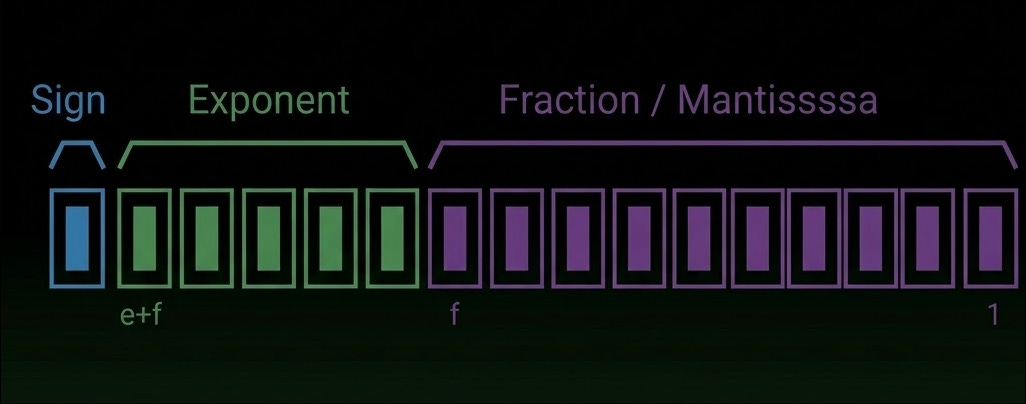
The IEEE 754 standard defines how floating-point numbers are represented and computed in modern hardware. Each number is encoded as three parts: a sign bit, an exponent (which determines dynamic range), and a mantissa (which determines precision).

These bits are interpreted as:

value = (−1)^sign × mantissa × 2^exponent

This can be generally thought of as sign sets the direction, exponent sets the scale, and mantissa sets the detail within that scale.

The FP32 format

The most popular of these datatypes are FP64, FP32 and FP16, using 64, 32 and 16 bits respectively.

Modern narrow datatypes

More recently there’s been a push to invent even more narrow-precision datatypes: BF16 from Google Brain, and more recently FP8 (E3M4, E4M3) and various 4-bit variants (MXFP4 and NVFP4).

The majority of the performance gains shown in more recent generation GPUs stem directly from using lower-precision datatypes, as seen in Nvidia’s gen-to-gen performance chart:

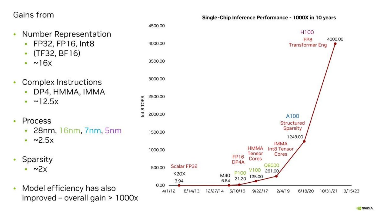
It is advantageous to use datatypes that require less bits because they take pressure off memory bandwidth, fit into caches better, and require fewer transistors to implement mathematical operations in hardware. However as we’ll see there are correctness tradeoffs associated with lower-precision datatypes.

We’ll talk more about TF32 later, as it’s an unusual case.

The precision spectrum

We now see a spectrum of datatypes:

• FP32 is the gold standard for precision and correctness (FP64 isn’t widely used in AI). Generally low-performance, high-correctness.

• FP16 / BF16 being a generally safe / mature format to use depending on if range or precision are targeted.

• FP8 for speed-of-light performance on Hopper-generation (2022 onwards) accelerators with some (manageable) accuracy tradeoffs and no block-scaling complexity.

• MXFP4 / NVFP4 for state-of-the-art performance on Blackwell-generation (2025 onwards) accelerators utilizing very low-bit weights for maximum bandwidth efficiency and scaling factors for preserving accuracy.

• INT8 is less commonly used in datacenter accelerators but common on edge devices owning to the simplicity of integer arithmetic hardware.

Sources of error

The tradeoff of a low-bit datatype is less representational power since fewer bits means fewer states. Fewer exponent bits shrink dynamic range resulting in more overflows and underflows, while fewer mantissa bits increases rounding errors.

Two additional behaviors also incur a mismatch between represented and real numbers: subnormals and flush-to-zero behavior. In IEEE 754, numbers very close to zero are represented using subnormals. Instead of the usual “1.xxx × 2^e” form, they drop the implicit leading 1 and use “0.xxx × 2^emin”. This allows gradual underflow where values don’t jump straight from the smallest normal number to zero, instead tapering off smoothly. Flush-to-zero is a performance optimization where the system treats all subnormal values as exactly zero, which eliminates the hardware required to correctly handle subnormal values.

These tradeoffs are tricky to track since they depend greatly on not only the datatype and hardware in question, but the exact operation as well, with some operations being much more sensitive to low-bit mismatches than others.

Accumulations are the most common source of errors, putting pressure on numeric precision for long accumulation sequences. While multiplications are generally fine to do in fairly low precision due to errors being finite and bounded, as the length of the accumulation grows, errors build up.

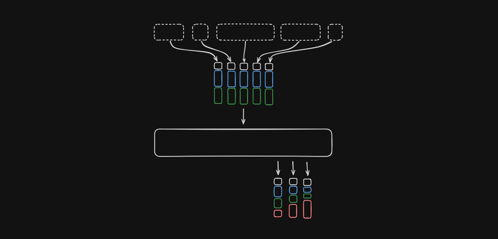
This is a big problem for matrix multiplies, which famously do long accumulation chains as part of their dot-product operation:

In the diagram above, we are taking a dot product of the elements in the shaded areas of the A and B matrices to get the single element shaded area of the C matrix. When the K dimension is large we need to do a long accumulation chain to get to the final result. LLMs have been increasing the K dimension for years, some now as large as 14848 in the case of Falcon 180B. For this reason most accelerators implement accumulators in a higher precision than the multiply units, often times as high as FP32.

Softmax is another common operation for errors to occur due to the exponentiation involved on every element, which increases the magnitude of each element and leads to common overflows, especially on low-exponent datatypes. Techniques like stable softmax involve subtracting the maximum element from all elements first before the standard softmax is applied for this reason.

\(softmax(x_i) = exp(x_i - max(x)) / sum(exp(x - max(x))))\)

Normalization, such as LayerNorms found inside most LLMs put high pressure on the precision (mantissa bits) when computing variance. On datatypes with low mantissa bits, rounding errors commonly occur. For this reason variance is often computed in FP32.

Outliers are a very common phenomena where a few elements in the activations dominate the scaling of an operation in a transformer and ruin the effective resolution in INT8 precision. Clipping activations can help eliminate outliers, however clipping fundamentally destroys information, so it also contributes to quality loss.

A note on determinism

AI models are generally made up entirely of linear algebra operations, and since linear algebra is generally thought of as deterministic, it stands to reason we can always get deterministic, reproducible outputs out of our AI models. Unfortunately as Thinking Machines has documented excellently here, that isn’t usually the case. Their post is very detailed and I would highly recommend reading it, but for our purposes I’ll summarize a key cause of nondeterminism as this inequality when dealing with finite-precision floating points:

\((a+b)+c \neq a+(b+c)\)

In modern floating-point hardware, such as GPUs, there are no guarantees made about accumulation ordering, meaning if the above holds true then we cannot be bit-wise certain about our outputs.

Hidden Precision

One major change to Nvidia GPUs over the past few generations (since Ampere in 2020) was the introduction of TensorFloat32 (TF32) precision. Despite the name, it actually uses 19 bits, specitically arranged as 8 exponent bits and 10 mantissa bits. You’ll notice this is essentially a mix of FP16’s mantissa (10 bits) and BF16’s exponent (8 bits), which gives it the same precision as FP16 and same range as BF16.

Even more confusingly, users never actually “touch” this datatype, meaning it isn’t meant to be directly handled in user code at all. You’ll never see a buffer of TF32 values or need to compute 19 * n_elements to determine a buffer size. Instead, it entirely exists within the TensorCore’s systolic array (matrix multiply unit) and enables much higher performance than native FP32 mode, albeit at the cost of less numerical precision. It is enabled or disabled in cublas with the arguments CUBLAS_TF32_TENSOR_OP_MATH or CUBLAS_DEFAULT_MATH respectively.

Quantization methods

Using fewer bits is only half the story, how you map values into those bits matters just as much. Quantization takes a high-precision value and maps it into a smaller set of discrete levels, typically via a scale:

q = round(x / scale)
x̂ = q * scale

Choosing that scale is where most of the tradeoffs live.

Per-tensor vs per-channel

Per-tensor uses one scale for an entire tensor. This is simple, but inaccurate if values vary widely.

Per-channel / per-block assigns a scale per row/column. This adapts much better to real distributions and is widely used despite slightly higher overhead.

Certain newer datatypes like nvfp4 mix these techniques, using a higher precision per-tensor scale and a lower precision per-block scale.

Static vs dynamic

Static quantization precomputes scales (common for weights).

Dynamic quantization computes them at runtime (common for activations).

Block-wise quantization

At very low bitwidths (FP8, 4-bit), scales are often shared across small blocks (e.g. 32 values). This improves accuracy but adds complexity and requires kernels to load both values and scales.

“Automatic” mixed precision

Since we’ve seen how certain operations are more sensitive to low-precision datatypes than others, couldn’t we just mark the operations that are sensitive and switch to high-precision datatypes for just those?

Yes! That’s exactly how PyTorch’s Automatic Mixed Precision works. It relies on a table that marks operations which require higher precision and does upcasts before and downcasts after. This helps to alleviate the primary issues of precision loss, though it’s a fairly brittle approach. As opsets are large, this is a large manual effort to make sure all operations are correctly marked, and when new operations are added, they can just as easily slip through this manual marking process and execute in a precision lower than is required for stable results.

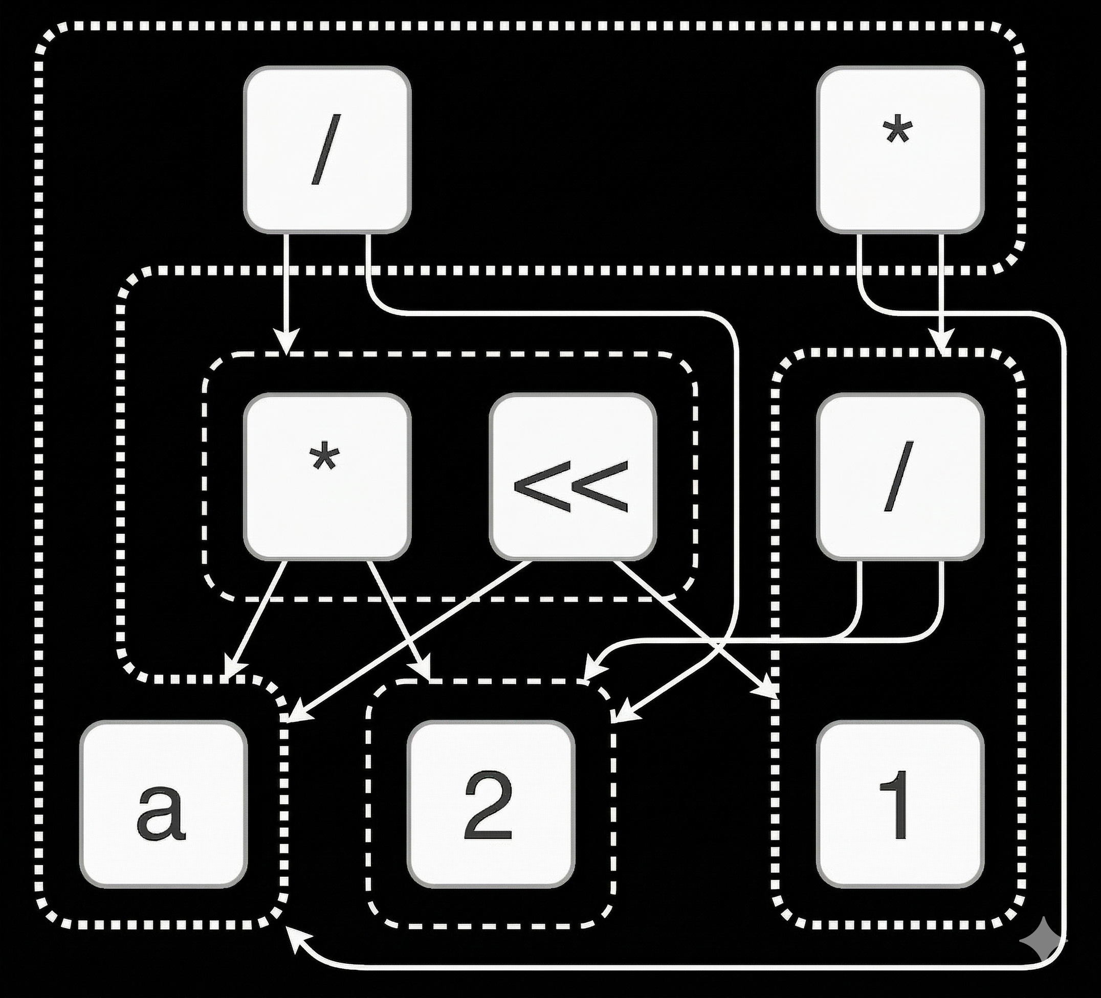
The compiler’s role in protecting accuracy

This manual op-marking approach starts to break down as we move towards a world of ML compilers, where the program written by the model developer is ingested into a compiler and undergoes aggressive optimizing transformations to reduce memory pressure or fit hardware units better. Operations that were previously insensitive to precision errors could be transformed into sensitive operations, or vice-versa. Compounding this, most compilers now operate at a lower level than whole tensor operations, meaning loops and blockwise or elementwise operations are tracked explicitly. For example, this means accumulations are often done in 2-step fashions, first accumulating inside a block and then accumulating between blocks, sometimes in different precisions. As we’ve seen before, long accumulation chains are hotspots for numerical error buildup.

In this world, its the compiler’s job to maintain a contract with the user: numerical error must not increase due to optimizations, or it must increase in predictable, user-controllable ways.

If this contract is not maintained, outputs end up being lower quality due to numerical errors / instabilities. Debugging this is a very involved process, often requiring a deep dive into the compiler’s internals and chosen transformations. Without good tooling, this is quite a challenging issue to debug!

Modelling precision in Luminal

An e-graph datastructure, like the one used in Luminal

Keeping this contract is vital to correct results, and given Luminal is a compiler focused on formal large scale search, we needed to be able to verifiably hold numeric guarantees even as the compiler traverses a semantically rich search space at various levels of operators.

A straightforward approach is to measure absolute tolerance (atol) error and relative tolerance (rtol) error end-to-end through an entire model. This is a standard technique used by many libraries, and works fairly well given sufficiently noisy inputs. However this approach has some drawbacks, most notably to do with runtime. We may have millions of compute graphs that would lead to unacceptable numerical losses, but this approach would require we ran each one fully to rule them out, a process that could take far too long at compile time.

An approach Luminal commonly uses is to do operator-level or subgraph-level precision tracking, essentially measuring operator or subgraph numerical errors and reasoning about how they compound in a whole model. One way to think about this is that if subgraph A has been measured (through atol and rtol) to produce unacceptable numerical loss, we can safely rule out all compute graphs that contain A, knowing that the remainder of the graph cannot have "less” overall error (this doesn’t hold true in a handful of edge cases, however this post is long enough!).

Static analysis represents another approach to quantifying errors in linear algebra expressions. There are several forms, but generally these take the form of:

• Start with bounds on input variables [a, b]

• Derive correlations through the expression and across operators

• Estimate overall error bounds

• Use a rewriting system to minimize error given some constraints

A common drawback to interval-based tracking is the explosion of error bounds. In order to guarantee outputs will fall within an interval, solvers will generally estimate worst-case on each operation, which builds up over the course of a full expression, leading to the end error interval overestimating the true error bounds.

Solvers like Daisy use bit-level representations to analyze bit-level transformations and symbolically model errors rigorously. The upside of this level of rigor typically is tighter end error bounds, without as much overestimation as general interval-based tracking. However due to bit-level tracking, these solvers can become quite expensive on large expressions (which LLMs certainly qualify as).

Generally static / analytical solvers are required to over-assume a worst-case error, and mixing in empirical error measurements with representative inputs often helps keep the search grounded to real-world data.

Wrapping up

Numerics determine whether your tokens can be trusted or not. Despite labs sinking billions into training better and better models, relatively little attention is paid to making sure the fidelity of those models are preserved after the benchmarking runs are over and they go into service.

As we’ve seen, modern computers can only represent floating point numbers with a finite number of bits, and so numerical error is unavoidable. Quantifying and controlling that error is vital. As Luminal is a compiler, it is our job to ensure no optimizations or rewriting destroys numerical accuracy, lest our outputs be not only fast but also incorrect.

General-purpose rewriting solutions, like those used in Luminal, allow us to traverse this space smoothly and reason about not only performance but also numerics in a joint space.

I’m excited about the possibilities of controllable, low-precision, low-error accelerated inference. Luminal exists in a unique space where we can co-design with our hardware partners and model partners to continue driving the cost of intelligence down, so when the “country of geniuses in a datacenter” arrives, we can all afford to use it.

If this excites you, we’re hiring.