

Introduction
The goal of this blog is to gain a better intuition over the tradeoffs of speculative decoding as applied to models like DeepSeek v4.1 Flash or GLM 5.3 Flash and to better understand the speculative decoding results here.

On Speculative Sampling
At base, speculative decoding (spec-dec) uses a smaller, more efficient draft model to generate n additional tokens, which are then verified by the target model. The thing which is maybe not immediately obvious is how we can sample those tokens from the draft model while still guaranteeing that our final output looks exactly as if we had sampled from the target model alone. This is what standard speculative sampling, as defined in the original spec-dec paper, gives us.
With the draft distribution q and the target distribution p, the drafter will propose some token x with probability q(x), and we will accept that proposal with probability
And before even thinking about rejection, we can ask how much probability this “accepted proposal” path contributes to token x.
And so the accepted proposals give us exactly the probability mass where p and q overlap.
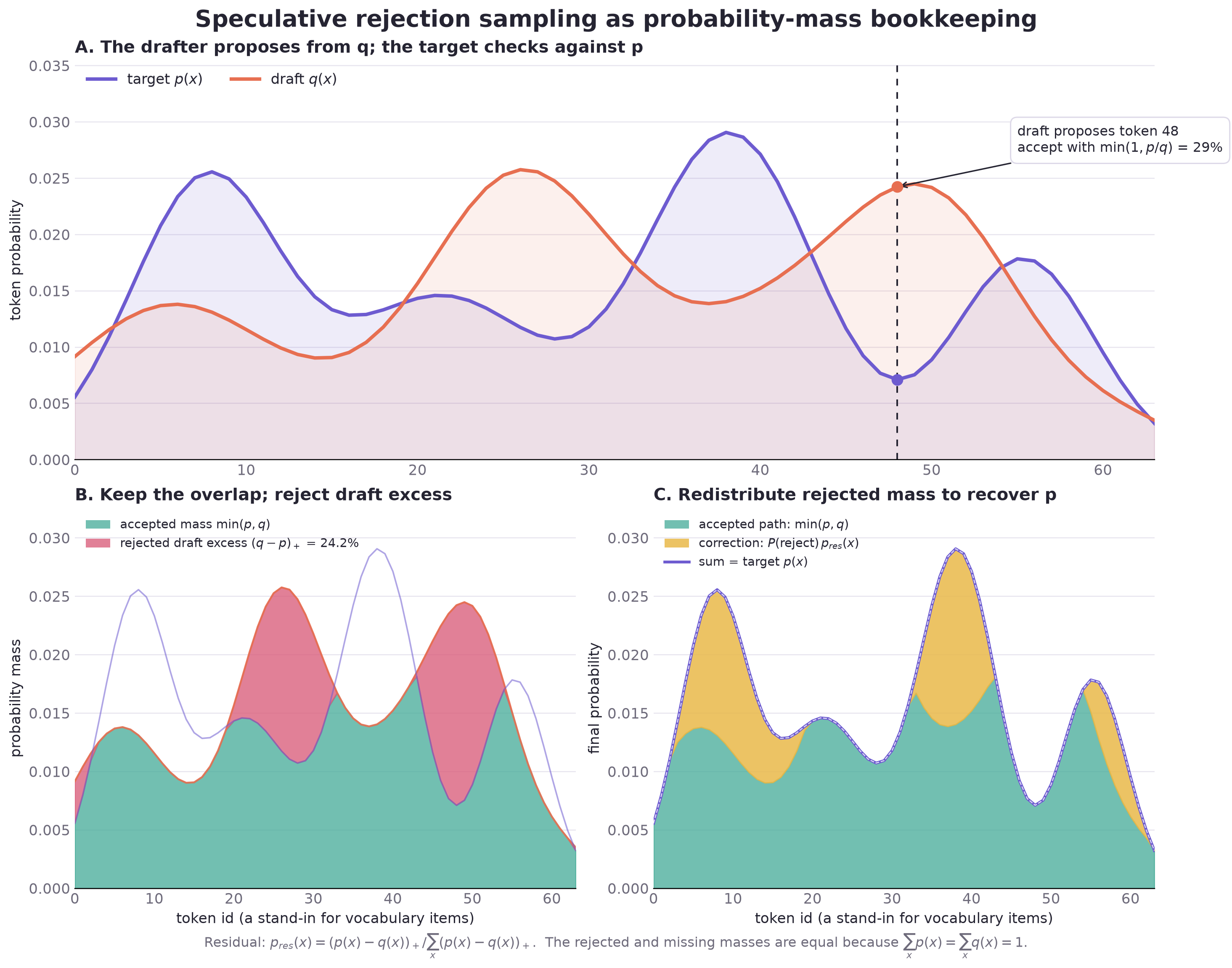
Panel A shows the two possible cases. Around token 40, p(x) > q(x), and so we accept every time. The drafter proposes this token less often than the target would have, meaning all of the probability supplied by q can safely be kept. Token 48 is the inverse case. Here q(x) > p(x), meaning the drafter proposes this token too often and we cannot accept every proposal. Eyeballing the graph gives us p(48) = 0.007 and q(48) = 0.025, and so we accept token 48 around 0.007 / 0.025 = 28% of the time.
We still need to account for the proposals we reject, which is what panels B and C are showing. Panel B is the excess probability supplied by the drafter. Across the complete vocabulary, we reject
Panel C shows where the rejected probability needs to go, where we can obtain the “missing” probability as
Which is the amount rejected in Panel B. We then sample the correction token from places where q came up short in proportion to how much probability mass is actually missing
The denominator is the total probability missing from q, which we just saw is also the chance of rejecting a proposal. Now, r(x) tells us how often we choose x among the proposals we rejected. To find how often we emit x as a correction overall, we multiply by the chance of rejection, which cancels that denominator. This leaves max(p(x) - q(x), 0), the probability q was missing for x, and if we add the probability of proposing and accepting x, which is min(p(x), q(x)), we get p(x).
Block verification
The DeepSeek v4.1 Flash recipe on vLLM, however, does not use standard token-by-token rejection sampling, and instead opts for block verification. Whereas standard verification stops at the first rejection, block verification checks all prefixes and keeps the longest passing one.
The block verification paper provides a toy example with two possible tokens. The drafter assigns q(A) = 2/3 and q(B) = 1/3, while the target assigns the opposite probabilities. These probabilities are the same at every position, so an A has a target-to-draft ratio of p(A) / q(A) = 1/2, while a B has a ratio of p(B) / q(B) = 2.
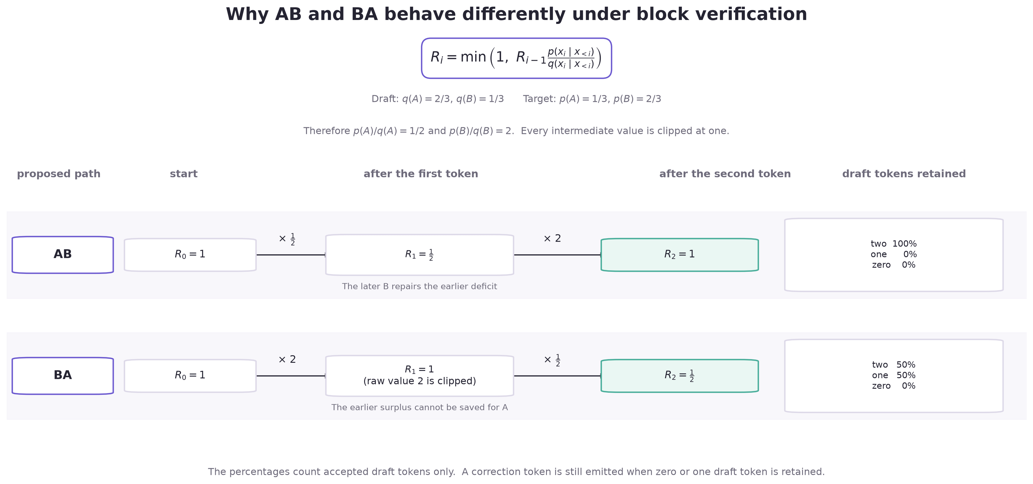
Now suppose the drafter proposes A B. Standard verification tests A first and rejects it half the time, but never gets to B, however, the complete A B sequence has probability 2/9 under both p and q, and so looking only at the first token misses that.
The picture keeps track of a running target-to-draft ratio. It starts at (probability) one, then gets multiplied by p(x) / q(x) for each proposed token, capping the result to one after every step. For A B, the A takes it down to 1/2 and the B brings it back to one. For B A, the B tries to take it up to two, but it gets capped at one before the A brings it down to 1/2. So the later B can make up for the earlier A, while a B that comes first cannot bank that extra probability for later.
This lets block verification keep all of A B even in cases where the first A would have failed the standard token-by-token test, and the verifier uses separate acceptance thresholds and correction sampling to make sure the output still follows p.
Adaptive verification
Even though DSpark might propose k tokens for each request, vLLM does not necessarily need to validate all of them, or even any of them. If we have some high degree of confidence that the token will not be accepted, it makes little sense to spend compute time validating it.
To help to facilitate this, DSpark ships with a confidence head that predicts whether each proposal will be accepted. And if the drafter doesn’t have a confidence head, vLLM watches what gets accepted while serving requests and learns how much to trust the drafter at each position.
vLLM also needs to know how much work those extra rows will cost. So, on startup, it times drafting for r requests and target verification for t rows, which we’ll call D(r) and V(t). For each possible number of verification rows b, vLLM picks the b draft positions most likely to survive and estimates whether checking them is worth the time.
That gives us the expected tokens per unit time, so vLLM picks the budget with the highest result.
Our own simple cost model
Let’s now move to speaking to what actual speedups we might see from using (fixed-depth verification) spec-dec. First defining some parameters:
C_0 = the time for one ordinary target-only decode step
D_k = DSpark's cost for producing `k` proposals (the default speculator used for DSV4.1 in vLLM)
V_k = the target model's cost for verifying those proposals and producing the next token
C_k = D_k + V_k, the complete cost of one speculative step
L_k = the expected number of tokens emitted by that speculative step
p_j is the unconditional probability that draft slot j is actually emitted by the speculative step, so
where the 1 is the correction or bonus token that the target contributes to the step. And the speedup, compared to ordinary decoding, can be given
So, figuring out whether or not adding another proposal helps, we can compare throughput with k proposals
against throughput with k+1 proposals
Here p_(k+1) is defined as the probability that the speculative step actually emits the token in slot k+1. So, adding one more speculative token will improve throughput when
Said plainly, the next token does not have to be accepted every time, but merely accepted often enough to pay for the drafting and verification.
The Role of Arithmetic Intensity
Arithmetic intensity is the amount of computation we do per byte from memory. While not a silver bullet in helping us to determine what another speculative position might cost, it can help build an intuition.
For instance, take a projection whose weights are much larger than its activations. With only a few query rows, much of the time goes into simply loading the weights, so adding another row lets us reuse the weights, doing more computation without reading much more from memory. At some point, once the projection becomes compute-bound, another row added means more matrix multiplication that the GPU actually has to spend time on.
On the other hand, for a different reason, attention can be bandwidth-bound. If the next query uses KV we’ve already read, then that extra row might be cheap, but if it makes us fetch a lot more KV, memory bandwidth makes that row quite expensive. The useful question then for speculative decoding then is what another token makes us read and compute.
DeepSeek v4.1’s Attention
Given all of whats above, what we are really after is, in the regime of DSV4.1, how adding draft proposals effects C_k, the time per speculative decode step.
Much of the internals of DS v4.1’s attention have been discussed elsewhere so I won’t go deeply into its actual architecture, but in general, we can say that its attention cost is
Looking at the config itself, we can say
based on which layers contain which types of attention.
Starting with the projection, if we assume inputs = [Q, H] and weights = [H, W], then we have QHW multiply-accumulates or 2QHW FLOPs. Memory movement has us read both QH and WH elements and write QW elements, so the arithmetic intensity becomes
Increasing Q amortizes the fixed weight read, so arithmetic intensity initially rises quickly, though eventually activation traffic dominates.
Next, for sliding window attention, for speculative position j, the SWA history has
positions. Simplifying a bit, let’s say FLOPs at some position j is 4 B n_h d W_j where we have B sequences, n_h query heads, with per-head dimension d, and the 4 coming from the qk dot product and accumulation both costing 2d FLOPs. Across q = k + 1 target query rows, the FLOPs are therefore
or approximately
once the window is full.
On the memory side, we’ll call b_KV the bytes needed for the K and V values of one cached position for one sequence. Assuming that the KV overlaps across sequence positions and so is loaded once and reused, the union of their windows contains around 128 + q - 1 positions, and so
And this gives
And if q is small relative to 128, this is approximately
which is why arithmetic intensity initially grows almost linearly as we speculate more tokens.
Finally, compressed sparse attention, and iIn some sense sparse attention is similar to sliding window attention. A candidate stage will first narrow the compressed history to 2,048 blocks of eight, after which the indexer will select 512 compressed latents for each query. The issue in terms of memory reuse is that the 512 positions selected for one token may overlap very little with those selected for the next. Ratio-2 layers do reduce the size of the compressed cache by pooling pairs of consecutive tokens into one KV latent, but they still don’t guarantee that different queries retrieve the same latents. In the non-ideal case, each speculative token produces different top-k sets, which causes compute and memory to grow with q and leaves arithmetic intensity close to constant. This gives us less reuse with which to make the additional rows cheap, and so every proposal still needs to produce enough additional output to pay for a roughly proportional increase in attention work.
DeepSeek v4.1’s MoE
DeepSeek’s MoE routes a given token to 6 of 384 routed experts, in addition to one shared expert which every token uses. Given (idealistic) uniform and independent routing, if N is the total number of routed experts and each token routes to r of them, the expected number of experts touched by Q query rows is:
Implying:
Query rows Q    Experts touched
------------    ---------------
1                         1.6%
4                         6.1%
8                        11.8%
16                       22.3%
32                       39.6%
64                       63.5%
96                       77.9%
128                      86.7%
192                      95.1%
256                      98.2%
384                      99.8%
512                     99.97%
What this means is that only around 300 to 400 query rows will nearly every routed expert be represented somewhere in the batch, which gives the MoE implementation the opportunity to reuse expert weights across multiple tokens. True, the number of experts touched is not really the quantity we care about, what matters more is how many token rows each expert actually receives, but even at Q = 384, our uniform model only gives six assignments per expert on average.
The separate MoE regimes can be somewhat decomposed. For small Q, new tokens activate new experts, so both the weights and FLOPs grow. For medium Q, as nearly all experts are represented, a kernel may be able to amortize those weights across more tokens. For large Q, expert compute or communication then becomes limiting and runtime grows more directly with the number of tokens.
DSpark Architecture
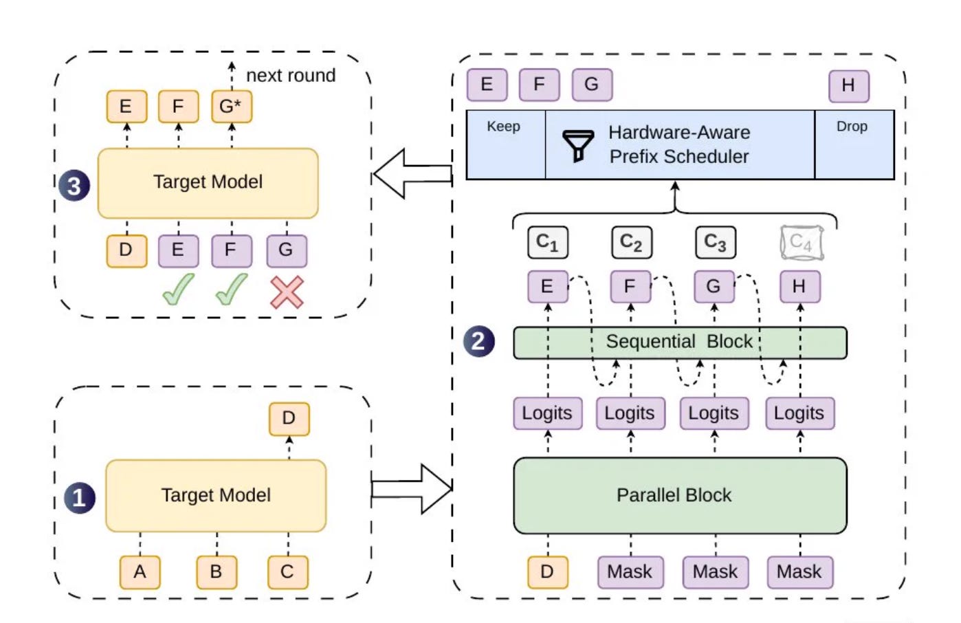
DSpark will take the hidden states from target layers 37, 38, and 39, project them back into the model dimension, and then run three draft layers over the entire speculative block in one diffusion-style parallel forward pass. The backbone then predicts all of the positions together, then a Markov head samples the block from left to right, using the previously sampled token to adjust the logits for the next position. There is also a confidence head that can be used to determine how much of the block is worth verifying.
Much of what we’ve already spoken about can be applied directly to DSpark’s cost. If DSpark processes something like Q_d = B * kdraft tokens, then (very coarsely) we can say
Moving from k to k+1 buys us only p_k+1 additional expected tokens, while increasing both the drafting and target verification cost. DSpark’s diffusion-style parallel backbone is meant to keep the first (drafting) part small, producing the whole block in one pass so that proposals we never use are relatively cheap to have drafted.
GLM 5.3 Flash as a comparison
The analysis above is deliberately centered on DeepSeek, but in our experiments we use GLM 5.3 Flash as a comparison. In terms of architectural differences, GLM uses one MTP layer rather than DSpark’s three layers, it uses both recurrent linear attention layers and sparse-attention layers, and its MoE routes a token to 8 of 288 experts plus one shared expert. We should definitely expect its drafting and verification curves to have different shapes, but we can still ask exactly the same questions about whether the probability of emitting another token is worth what that additional position costs.
Experiments
We ran DeepSeek V4.1 Flash with DSpark and GLM 5.3 Flash with MTP, with each server using four B300s under TEP4. For each model we tested k = 0...5, 18 decode batch sizes from B = 1 through 256, starting contexts of 512, 8192, and 32768, and several acceptance profiles from reject-all to accept-all. Every point was repeated with the GPU lanes swapped and the prompts held fixed.
The metric is accepted decode output tokens per second with exactly B active requests and no prompt work or request turnover. It is not end-to-end throughput for a mixed production workload. Both coding runs used block verification, while the synthetic surface used vLLM’s synthetic verifier to force the per-position acceptance rates.
We used AIPerf for both workloads. The synthetic runs processed every prompt before measuring a fixed cohort of B decoding requests. The coding workload replayed the length distribution of a 500-request production trace at concurrency 96, and so its active decode batch varied as requests finished.
The faint dots that you can toggle in the UI are the actual benchmark runs. The colored lines interpolate between their measured acceptance profiles, which lets us change the acceptance curve and estimate throughput across the batch-size grid.
To explore the interactive speculative decoding results click the image or here and to check out our pull request that added adaptive verification support to vLLM click here.
Conclusion
The best speculative depth is the depth at which another position stops paying for itself given the workload we’re serving. The experiments give us a sort of price for each additional speculated token, while adaptive verification lets the target decide how much of that price each request should actually pay.
But this price only belongs to the particular regime we measured. When actually serving, changing the number of speculated tokens can change the batch shape, CUDA graph selection, padding, memory pressure, concurrent requests, and so on, which makes the architectural arguments only a rough guide. The best value of k therefore is not a property of the drafter alone, but of the complete serving system.
