
Compiling Models to Megakernels
Fine-grained synchronization, deep pipelines, and zero kernel launch overheads, automatically.


Luminal is an inference compiler, and as such we’re interested in driving inference right up to the physical limits of the hardware. Inference has two fundamental limitations: compute (flops) and bandwidth (TB/s). Increasing these two requires buying much more expensive hardware, so we want to make sure we’re using all the compute and bandwidth we have available to us! This basically boils down to: anytime the GPU is not loading data, we’re wasting bandwidth, and anytime the GPU is not computing, we’re wasting compute.
Bottlenecks
Let’s look at a typical timeline of executing a transformer layer:
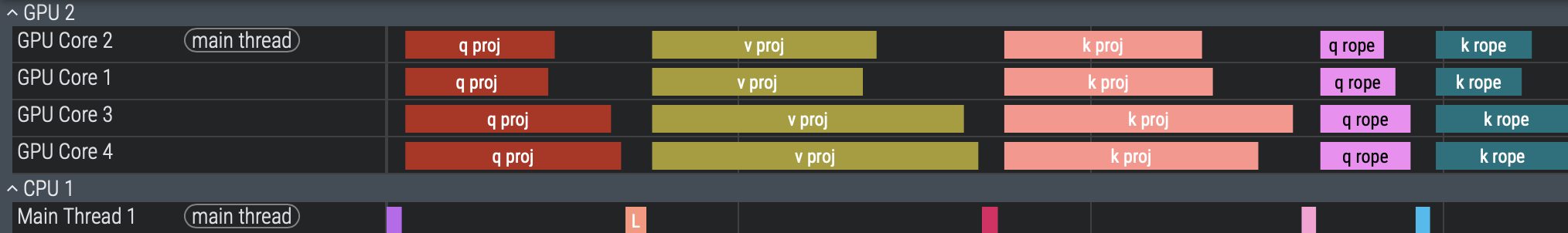
We see two problems immediately:
Every time we finish a kernel and start another one, the GPU sits idle while the CPU launches the next kernel.
Some streaming-multiprocessor cores (SMs) in the GPU finish their work early and sit idle while other SMs finish the remaining work.
Kernel launch overhead is well-known and can be partially mitigated with techniques like CUDA Graphs on Nvidia GPUs. This isn’t perfect, though, as Hazy Research demonstrated in their original megakernel post. With a dummy kernel that does no work, and ordinarily takes 2.1 micros, when CUDA graphs are enabled, it still takes 1.3 micros!
The next issue is also a well-known phenomenon called Wave Quantization, which occurs when a kernel’s work cannot be evenly distributed across all SMs, leaving some SMs to finish early and stall while others lag behind to finish the kernel. Depending on the total runtime of the kernels and the shape of the work, these gaps can become very significant!
Due to the nature of the tensor computations we’re interested in, we don’t actually have to wait for a full synchronization to begin the next op. Take a tiled matmul for example:

This operation does not need to wait for all of tensor A or all of tensor B to begin computing, since it only consumes a stripe of tiles from both A and B. So long as that stripe is ready, we can start computing a tile of C! This full synchronization is entirely enforced by the standard kernel execution model, not required by the mathematics.
There’s actually a hidden third bottleneck preventing us from fully utilizing our hardware’s bandwidth and compute effectively: each kernel does no compute until it loads enough weights to start working. Generally this means even if the kernel can do perfect load-compute overlapping during it’s main loop execution, it cannot get around the idle time waiting for the initial weights to load. We’d need a finer-grained timeline showing loading and compute to see that effect:
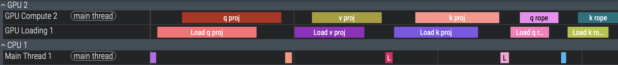
Now we can see there’s a large amount of time spent loading the initial weights before we can even begin to compute. The whole time our expensive tensor cores are sitting idle! Even if our kernels were programmed by experts and perfectly utilized bandwidth during their execution, this is outside their control. Techniques like Programmatic Dependent Launch help mitigate this by letting the next kernel start setting up (loading weights) while the current kernel is running, however this is done on the device level, not the per-SM level, so we’re still left with significant bubbles.
One kernel per model
What if instead we could fuse every operation in a forward pass into a single kernel? This would give us a few advantages:
We’d eliminate kernel launch latency right off the bat, since we only launch one kernel for the entire forward pass.
We’d also be able to immediately start running work from the next operation on SMs that have early-finished work on the current operations, eliminating our wave quantization effects.
We’d be able to start loading weights for the SM’s next operation during the epilogue of the current operation, thereby eliminating the above gap between compute spans.
This technique was pioneered by Hazy Research last year, where they fused Llama 1B into a single megakernel. However, a significant limitation of their approach was requiring these megakernels to be built by hand, manually defining each instruction and scheduling it to SMs. Since we’re compiling models from source, we want this process to be automatic and robust to arbitrary architectures.
Let’s walk through how megakernels work, and then we’ll dive in to how Luminal automatically generates them for arbitrarily complex models.
An interpreter on a GPU
Megakernels stem from the concept of an interpreter. Most programmers will be familiar with how interpreted languages like Python work, where an interpreter reads, decodes, and executes instructions one-by-one. We can view a GPU as a large multi-core processor, where each core is capable of executing a very limited instruction set. We can either provide the cores their instructions directly in shared memory on a per-core basis, or in global memory in a global instruction stream. In other words, we need to decide if we want to statically schedule instructions to independent streams per-SM or on a single stream SMs all share.
A quick word about each path:
Static scheduling benefits from being able to prefetch and load many instructions at a time, directly into shared memory. The overhead for fetching a new instruction is very low since it’s already fetched at execution time and resides in fast memory. A downside of this approach is it requires the programmer or compiler to statically partition instructions across SMs ahead of time, which is challenging especially since instructions can be variable-latency. Furthermore, jitter is often present in SMs, causing some to run slower than others for unpredictable hardware reasons.
Dynamic (global) scheduling incurs more significant overhead by requiring a roundtrip to global memory and an atomic lock to fetch each instruction. These can be hidden though, during the execution of the previous instruction, so long as the previous instruction takes enough time to hide the fetch latency. Global scheduling also does not require the programmer or compiler to partition instructions to SMs ahead of time, instead allowing SMs to opportunistically pop instructions off the queue once they are ready. This naturally corrects for jitter, because faster SMs will pick up the slack while slower ones lag.
We felt the tradeoffs introduced with dynamic scheduling were worth it. Our megakernels provide a single global instruction queue shared by all SMs, which both simplifies the compiler’s work as well as allows for variable-latency instructions.
Since instructions communicate through global memory, we still want to do the same fusion patterns as in traditional kernels. This means our instructions end up being fairly coarse grained, handling computations like Matmul + ResidualAdd or RMSNorm + Matmul + RoPE to minimize global memory roundtrips.
Here’s a view of how our SMs work through instructions:
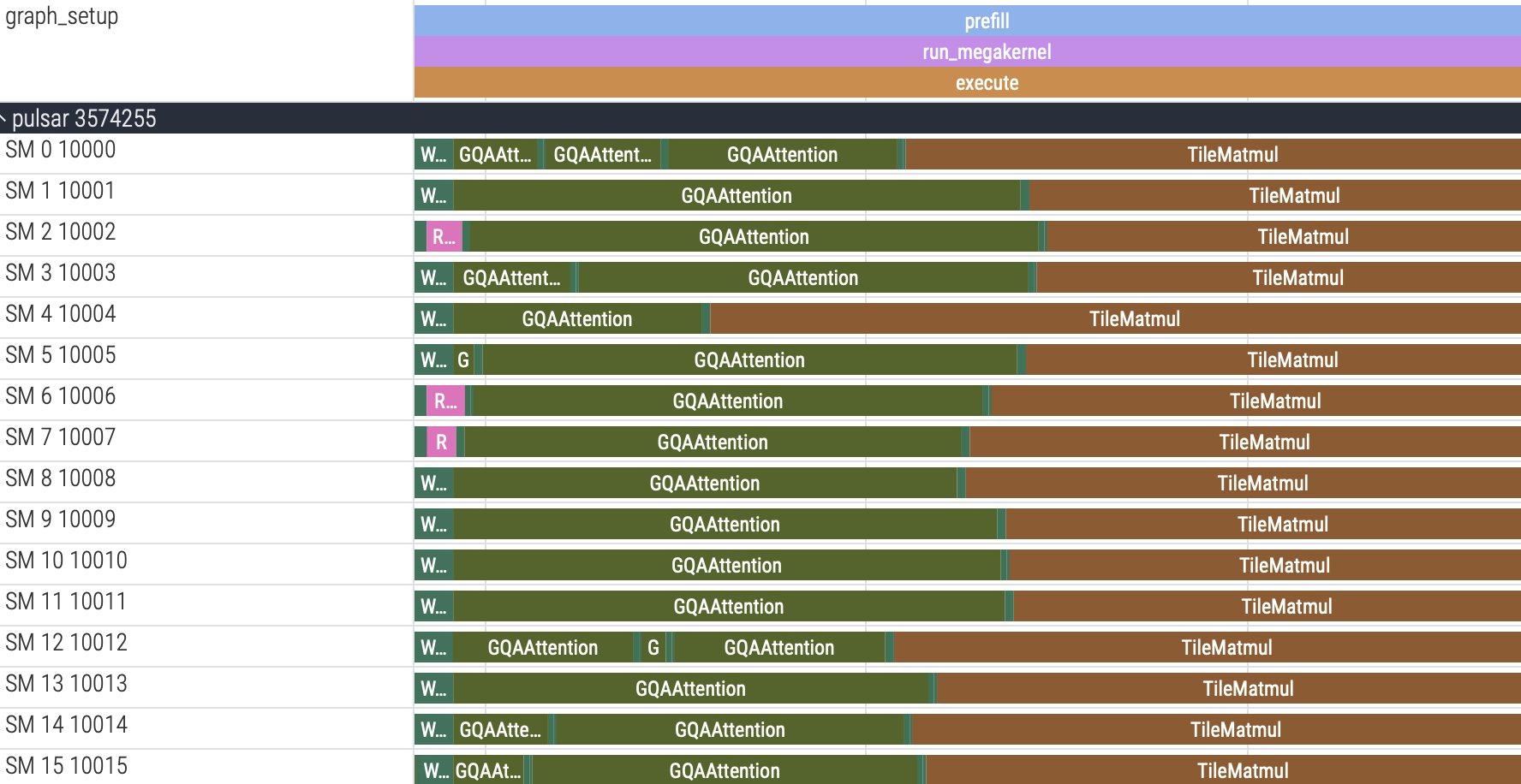
Notice how there’s overlap between when the current instruction ends and the next instruction begins running. We also even see SMs running multiple instances of instructions in the same timespan single instructions run on other SMs, showing that instruction latency is quite variable!
There’s one big problem left we haven’t discussed: synchronization. As we discussed before, normal kernels have a major downside in that future work cannot be ran until all SMs finish on the current kernel. However, the corollary to that is we are guaranteed all data is ready by the start of the next kernel. Once we start running future ops before past ops are entirely done, this guarantee goes away, requiring us to be very fine-grained in how we synchronize and assert the input data to the next op is in fact ready. The mechanism we use for doing this is standard barrier counters. However, unlike Hazy’s barriers, we use an increment-then-decrement barrier approach, where ops first increment their assigned barrier at launch, run, and then decrement their barrier once they are completed. We can then view each barrier as a sort of “inflight producer” counter. This mechanism means we don’t need the consumer to know how many producers to wait for on a given piece of data, it simply needs to wait for the number of inflight producers to equal zero.
Generating Megakernels
Luminal is a graph-based compiler, and as such it represents models as compute graphs. The challenge we undertake is transforming a compute graph into an instruction queue, with fine-grained data dependencies wired up correctly. Our approach takes 2 passes:
Rewriting existing ops into block ops, partitioned over SMs, with strided input and output data dependencies
Deriving barrier strides given all present input-output op pairings.
The first step is relatively straightforward. We have an op, say Matmul, that can be rewritten into a TileMatmul to handle a tile of data at a time. During the process of rewriting, we use shape-layout algebra (similar to CuTE) inside the e-graph engine (egglog) to derive correct strides for each input and the output tiles. Our approach is flexible on the shape of data we input and output from ops. For instance, some ops benefit from tiles (like matmul) whereas others don’t and operating on contiguous rows at a time is more efficient.
Once we have partitioned ops, we derive the barriers each op should consume from (check equals 0 before running) and produce to (increment and decrement). Let’s make this concrete by going back to our tile matmul example:
In this case, lets say M = 128, N = 128, K = 128, and our tiles are of size 32x32. We’re launching a 2D grid of (128 / 32) x (128 / 32) = 4 x 4 = 16 tile matmul instances to cover C. Our job is to work out the expression that would map the launch index (0-15) to a barrier index for source A. This is done by looking at the producer of A’s launch dimensions. If they are the same size along M we can prove independence along that dimension, since we only consume one tile’s worth of data along M. Therefore along M we initialize 128 / 32 = 4 barriers, and use a stride of 1 to specify that as we launch down that dimension, we want to step our barriers by 1. Along K we are always consuming the whole dimension, so our stride there should be 0. Therefore our final A barrier stride would be m * 1 + n * 0 or flattened along a single launch axis, it would be (x / 4) * 1 + (x % 4) * 0 = x / 4 , which maps our launch index (0-15) to our barrier (0-3) we want to consume from.
The idea behind analyzing each launch dimension is to preserve as much independence as possible. In the worst case, we need every producer SM and every consumer SM to share a single barrier, which would bring us back to the full-sync of traditional kernels. In the best case we have full independence where each next op depends on only one previous op, and can launch immediately when an SM completes.
This all ties together in a struct that looks like this:
struct BlockOp {
  src_a_data: Expression,
  src_b_data: Expression,
  src_a_barrier: Expression,
  src_b_barrier: Expression,
  dest_data: Expression,
  dest_barrier: Expression,
}
Where each expression defines a stride mapping the logical launch index to a physical index. Now each op knows where to get it’s source data, which barriers to look at before running, where to write it’s dest data, and which barrier to increment / decrement.
The next step is to generate the op implementations for all of these ops, from each block-op’s definitions. A standard implementation takes this form:
__device__ void mk_op(
    OpPayload payload, // op-specific payload struct containing metadata
    const float* const source_ptrs[3], // source data pointers resolved by the interpreter
    float* out_ptr, // dest data pointer resolved by the interpreter
    const int current, // the current logical launch index of this op
    int t // the current thread index in this threadblock
) {
    // body
}
This gives us all the information we need to execute a block op. The interpreter resolves the data pointers and barriers, correctly waits on barriers, and passes in data pointers to our implementation function. Ops also can create payload structs and place them in the instruction queue to be passed to the implementation. These structs typically have metadata in them, such as runtime dimensions or pointers to special data stores like external KV caches. By not constraining the metadata ops can access, we can get very creative with op design and access execution patterns not possible in more constrained implementations.
Symbolic Work Queues
One big challenge up front was how to handle rebuilding work queues (instruction queues) in between executions. The process of reallocating and re-scheduling every operation on a queue before each and every execution can be large and become a major bottleneck. Certain queues can be cached for multiple runs, but in general we don’t want to worry about the costly process of re-allocating and rebuilding queues every time something as simple as a sequence length changes.

Luminal’s solution to this is to represent instructions in the work queue, rather than instruction instances, we call this a symbolic work queue. For instance, if we have a MxKxN matmul that is partitioned into (M / 32)x(N / 32) tiled matmul ops, we don’t actually want to have (M / 32)x(N / 32) ops present in the queue. Instead we’ll put one tiled matmul entry in the queue and mark it’s launch dimensions as (M / 32)x(N / 32). Then we’ll initialize a running counter of how many remaining instruction instances we need to launch for the given instruction on the queue before moving the program counter. These will be atomically decremented as each SM pops another instruction instance off the queue.
What this gets us is an ability to symbolically represent how many instances of an instruction we want to fire off. For another example, let’s say we have a tensor of shape Sx128, and a row normalization op that normalizes a row at a time. We want to fire off S ops, which we represent exactly as such. Then at runtime we simply evaluate S with the concrete dynamic dimension values which contain the real sequence length for that execution, and we get the correct number of operations to dispatch. By representing our data pointers and barriers as strides, we can also do the exact same process of expression evaluation to resolve real data pointers and barriers at runtime. We can now change S (and any other dynamic dimension) with zero modification to the underlying work queue (or any other host-side work) at runtime!
All that’s left is to assemble the work queue once at compile time by topologically visiting each partitioned op, scheduling it’s instruction / payload struct, and then at runtime calling a single kernel dispatch and waiting on the results!
Conclusion
We’ve come a long way, so lets recap:
Traditional kernels cause bubbles through kernel launch overhead, wave quantization, and inter-instruction memory bubbles
By fusing an entire model into a single megakernel, we can overcome all three of these challenges
We can generate megakernels through a multi-stage process of rewriting an op to be partitioned over SMs, deriving data and barrier strides, and generating an interpreter by inlining each op’s implementation functions. Then we visit each op in the graph again to build the work queue, and bring the queue and interpreter together to execute!
It’s still early days for megakernels. A lot of abstractions have yet to be built, but we’re excited to realize a cleaner, more performant programming model for GPUs and custom accelerators focused on minimizing unnecessary synchronizations and keeping the hardware resources busy.
We’re releasing our work on megakernels in the Luminal compiler repo, come check it out and contribute. We’re leveraging the bitter lesson to build a truly next generation inference compiler, learning from decades of industry progress in ML, compiler engineering, and HPC. The future demands orders of magnitude more efficient compute. If this kind of state-of-the-art inference engineering excites you, we’re hiring! Shoot me a DM.
A big thanks to Hazy Research for their pioneering work in megakernels.
 | A guest post by
|
Hi Joe and Luminal, thanks for the great blog. We wanted to share our MPK project (https://github.com/mirage-project/mirage ), which is a compiler and runtime for mega-kernelizing LLMs using compiler superoptimization. We also have a paper describing the approach and results here: https://arxiv.org/pdf/2512.22219. We’d be very interested to see how Luminal compares with MPK, and would be happy to exchange ideas of course.